Animated Movie of Brain Data from Neuroscience using ParaView

Background

At FZJ, the institute for ​structural and functional organisation of the brain (INM-1) develops a 3-D model of the human brain which considers cortical architecture, connectivity, genetics and function. The INM-1 research group ​Fiber Architecture develops techniques to reconstruct the three-dimensional nerve fiber architecture in mouse, rat, monkey, and human brains at microscopic resolution. As a key technology, the neuroimaging technique Three-dimensional Polarized Light Imaging (3D-PLI) is used. To determine the spatial orientations of the nerve fibers, a fixated and frozen postmortem brain is cut with a cryotome into histological sections (≤ 70 µm). Every slice is then scanned by high resolution microscopes, resulting in a uniform rectilinear grid of scanned points.

The data used in this visualisation scenario consists of 234 slices of size 31076 x 28721 each, resulting in a rectilinear uniform grid of size 31076 x 28721 x 234 (~200 GB memory usage in total). Originally the data was stored as raw binary unsigned char data, one file for each slice.

Conversion to HDF5

Because ParaView has a well working XDMF/HDF5 reader, we decided to convert the raw data to hdf5 first. This was done using a Python script. Before Python can be used on our JURECA cluster, the necessary modules have to be loaded first:

module load GCC/5.4.0
module load ParaStationMPI/5.1.5-1
module load h5py/2.6.0-Python-2.7.12
module load HDF5/1.8.17

The Python-script scans the directory containing the 234 slice files for the names of the raw-files. Every file is opened and the raw content is loaded into a numpy array. This numpy array is written into the dataset of a hdf5 file, which was created first.

import sys
import h5py # http://www.h5py.org/
import numpy as np
import glob

dir = "/homeb/zam/zilken/JURECA/projekte/hdf5_inm_converter/Vervet_Sehrinde_rightHem_direction/data"
hdf5Filename="/homeb/zam/zilken/JURECA/projekte/hdf5_inm_converter/Vervet_Sehrinde_rightHem_direction/data/Vervet_Sehrinde.h5"

# grid-size of one slice
numX = 28721
numY = 31076

# scan directory for the filenames of the raw files
files = glob.glob(dir + "/*.raw")
numSlices = len(files) # actually 234 slices for this specific dataset

# create hdf5 file
fout = h5py.File(hdf5Filename, 'w')
# create a dataset in the hdf5 file of type unsigned char = uint8
dset = fout.create_dataset("PLI", (numSlices, numX, numY), dtype=np.uint8)

for rawFilename in sorted(files):
   print "processing " + rawFilename
   sys.stdout.flush()

   # open each raw file
   fin = open(rawFilename, "rb")
   # and read the content
   v = np.fromfile(fin, dtype=np.uint8, count=numX*numY)
   fin.close()
   v = v.reshape(1, numX, numY)
   # store the data in the hdf5 file at the right place
   dset[i, : , :]=v

print "success"
fout.close()

Creating XDMF Files

ParaView needs proper XDMF files to be able to read the data from the hdf5 file. We generated two xdfm files by hand. One for the fullsize dataset, and one for spatial subsampled version ('hyperslab').

The xdmf file for the fullsize dataset is quite simple an defines just the uniform rectilinear grid with one attribute named 'PLI'. It is a very good practise to normalize the spatial extend (size) of the grid by setting the grid spacing accordingly. We decided that the grid should have the extend "1.0" in the direction of its longest axis, which is 31076 pixels.
Therefore the grid spacing is set to 1.0/31076=3.21792e-5 for the Y- and Z-axis. The X-axis is the direction in which the brain slices have been cut and has a much lower resolution (by the factor of 40). Therefore it's grid spacing is 40 times larger, resulting in 40*3.21792e-5=1.2872e-3. The origin of the grid was set to its center.

Fullsize Version:

<?xml version ="1.0" ?>
<!DOCTYPE xdmf SYSTEM "Xdmf.dtd" []>
<Xdmf Version="2.0">
<Domain>
<Grid Name="Brain" GridType="Uniform">
<Topology TopologyType="3DCoRectMesh" NumberOfElements="234 28721 31076"/>
<Geometry GeometryType="ORIGIN_DXDYDZ">
        <DataItem Dimensions="3" NumberType="Float" Precision="4" Format="XML">
                 -0.151 -.4621 -0.5
        </DataItem>
        <DataItem Dimensions="3" NumberType="Float" Precision="4" Format="XML">
                1.2872e-3  3.21792e-5 3.21792e-5
        </DataItem>
</Geometry>
<Attribute Name="PLI" AttributeType="Scalar" Center="Node">
        <DataItem Dimensions="234 28721 31076" NumberType="UChar" Precision="1" Format="HDF">
                Vervet_Sehrinde.h5:/PLI
        </DataItem>
</Attribute>
</Grid>
</Domain>
</Xdmf>

As the dataset is relatively large (200 GB), we decided to generate a second xdmf file which only reads a subsampled version of the data (every 4th pixel in Y- and Z-direction, 12.5 GB). This is conveniant because the loading time is much shorter and the handling of the data is more fluent. The subsampling can be done via the "hyperslab" construct in the xdmf file and adds a little bit more complexity to the description. Please note that the grid spacing has to be adapted to the subsampled grid size, as we want that the spatial extend of the fullsize and the subsampled grid should be 1.0 in both cases.

Subsampled Version:

<?xml version ="1.0" ?>
<!DOCTYPE xdmf SYSTEM "Xdmf.dtd" []>
<Xdmf Version="2.0">
<Domain>
<Grid Name="Brain" GridType="Uniform">
<Topology TopologyType="3DCoRectMesh" NumberOfElements="234 7180 7760"/>
<Geometry GeometryType="ORIGIN_DXDYDZ">
        <DataItem Dimensions="3" NumberType="Float" Precision="4" Format="XML">
                 -0.151 -0.4626 -0.5
        </DataItem>
        <DataItem Dimensions="3" NumberType="Float" Precision="4" Format="XML">
                1.28866e-3 1.28866e-4 1.28866e-4
        </DataItem>
</Geometry>
<Attribute Name="PLI" AttributeType="Scalar" Center="Node">
    <DataItem ItemType="Hyperslab" Dimensions="234 7180 7760" NumberType="UChar" Precision="1">
        <DataItem Dimensions="3 3" Format="XML">
           0 0 0
           1 4 4
           234 7180 7760
        </DataItem>
        <DataItem Dimensions="234 28721 31076" NumberType="UChar" Precision="1" Format="HDF">
                Vervet_Sehrinde.h5:/PLI
        </DataItem>
   </DataItem>
</Attribute>
</Grid>
</Domain>
</Xdmf>

Prototyping the Movie

The final movie is generate by controlling the rendering process in ParaView via a Python-script (pvpython). Before this can be done, we need to identify good camera positions for camera flights, proper color- and opacity-tables, maybe a volume of interest, and so on.

To find out the necessary parameters, the data can be loaded and examined with the normal ParaView GUI first. Within the GUI the user can interactively adjust camera positions, color tables, and so on, in a very conveniant way. The obtained parameters can later be used in the final Python-script.
While prototyping the movie, it is also very helpful to open the Python-Trace window of ParaView, where most parameter changes (interactively made in the GUI) are shown as Python commands. These commands can, with minor changes, be used in the final Python script for the production of the movie.

Generating the Movie with Python Scripting

In the next sections the resulting Python script is shown step by step.

Preliminary Steps

First of all one has to import paraview.simple and open a view of the correct size (e.g. 1920x1080=fullHD or 3840x2160=4K). It is mandatory to switch on offscreen rendering, as else the size of the view would be limited by the size of the XWindow desktop.

#### import the simple module from the paraview
from paraview.simple import *

Connect() #connect to build-in paraview
# its also possible to connect to pvserver, e.g. pv.Connect('localhost')

paraview.simple._DisableFirstRenderCameraReset()

# get active view
renderView = CreateRenderView('RenderView')
renderView.UseOffscreenRendering = 1
renderView.ViewSize = [1920*2, 1080*2]

Loading the Data and Switching on Volume Rendering

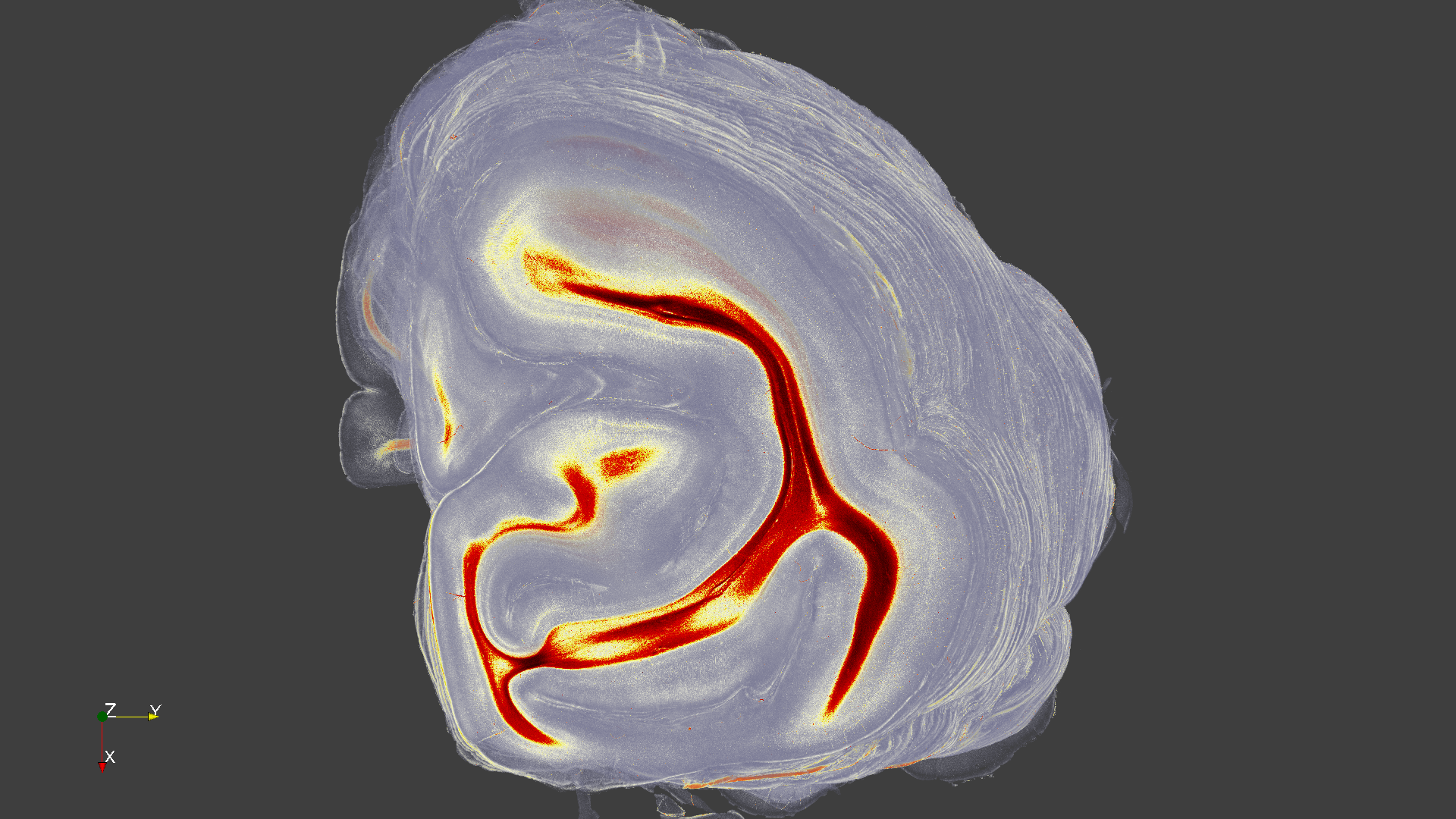
The data is loaded and then visualized with the ​OSPRay volume renderer. Proper color and opacity functions and a good camera position are set.

vervet = XDMFReader(FileNames=['/homeb/zam/zilken/JURECA/projekte/hdf5_inm_converter/Vervet_Sehrinde_rightHem_direction/data/vervet_hyperslab.xdmf'])
vervet.PointArrayStatus = ['PLI']
vervet.GridStatus = ['Brain']
print "loading vervet data"
vervetDisplay = Show(vervet, renderView)
vervetDisplay.VolumeRenderingMode = 'OSPRay Based'
vervetDisplay.SetRepresentationType('Volume')
vervetDisplay.ColorArrayName = ['POINTS', '']
vervetDisplay.OSPRayScaleArray = 'PLI'
vervetDisplay.OSPRayScaleFunction = 'PiecewiseFunction'
vervetDisplay.SelectOrientationVectors = 'None'
vervetDisplay.ScaleFactor = 0.09998712839442306
vervetDisplay.SelectScaleArray = 'PLI'

pLILUT = GetColorTransferFunction('PLI')
pLILUT.ScalarRangeInitialized = 1.0
pLILUT.RGBPoints = [0.0, 0.33, 0.33, 0.5,   27.0, 1.0, 1.0, .9,   51.0, 0.9, 0.9, 0.0,   65.0, 0.9, 0.0, 0.0,   254.0, 0.0, 0.0, 0.0]
pLILUT.ColorSpace = 'RGB'

# get opacity transfer function/opacity map for 'PLI'
pLIPWF = GetOpacityTransferFunction('PLI')
pLIPWF.Points = [0.0, 0.0, 0.5, 0.0,   254.0, 1.0, 0.5, 0.0]
pLIPWF.ScalarRangeInitialized = 1

camera = GetActiveCamera()
camera.SetPosition(0.0, 0.0, 1.488)
camera.SetFocalPoint(0.0, 0.0, 0.0)
camera.SetViewUp(-1.0, 0.0, 0.0)
Render()

Resulting Image:

Camera Animation: Path-based (Orbit)

To orbit around the data (rotate the data), the camera can be animated in 'Path-based' mode. In this example the CameraTrack and the AnimationScene are used in conjunction with two keyframes to render 100 images. Please note that in 'Path-based' mode the location of ALL camera positions on the track are stored in PositionPathPoints of the first keyframe!

cameraAnimationCue1 = GetCameraTrack(view=renderView)
animationScene = GetAnimationScene()

# create first keyframe
# Note: this one keyframe stores all orbit camera position in PositionPathPoints
keyFrame5157 = CameraKeyFrame()
keyFrame5157.Position = [0.0, 0.0, 1.488]
keyFrame5157.ViewUp = [-1.0, 0.0, 0.0]
keyFrame5157.ParallelScale = 0.6825949417738006
keyFrame5157.PositionPathPoints = [0.0, 0.0, 1.488, 0.0, 1.1563931906479727, 0.9364287418821582, 0.0, 1.455483629891903, -0.30937259593682587, 0.0, 0.6755378636124458, -1.3258177079922915, 0.0, -0.6052241248967907, -1.3593556409721905, 0.0, -1.437297629518134, -0.3851227391125512, 0.0, -1.2038172876299222, 0.8746244554111999]
keyFrame5157.FocalPathPoints = [0.0, 0.0, 0.0]
keyFrame5157.ClosedPositionPath = 1

# create last keyframe
keyFrame5158 = CameraKeyFrame()
keyFrame5158.KeyTime = 1.0
keyFrame5158.Position = [0.0, 0.0, 1.488]
keyFrame5158.ViewUp = [-1.0, 0.0, 0.0]
keyFrame5158.ParallelScale = 0.6825949417738006

# initialize the animation track
cameraAnimationCue1.Mode = 'Path-based'
cameraAnimationCue1.KeyFrames = [keyFrame5157, keyFrame5158]

numFrames = 100
imageNum = 0
animationScene.NumberOfFrames = numFrames
animationScene.GoToFirst()
for i in range(numFrames):
  print ("orbit state: rendering image %04d" % (imageNum))
  WriteImage("image_%04d.png" % (imageNum))
  imageNum = imageNum + 1
  animationScene.GoToNext()

Camera Orbit, resulting movie snippet (click on image to download movie):

Camera Animation: Interpolate Camera

For whatever reason, ParaView offers a second option for camera animation, called "interpolate camera". In this mode, the Position-, FocalPoint- and ViewUp-vectors of a given number of keyframes are interpolated. This way a camera flight consisting of 2, 3 or more keyframes can be animated. Here is an example for 3 keyframes.

cameraAnimationCue1 = GetCameraTrack(view=renderView)
animationScene = GetAnimationScene()

# create key frame 1
keyFrame1 = CameraKeyFrame()
keyFrame1.KeyTime = 0.0
keyFrame1.Position = [0.0, 0.0,  1.488]
keyFrame1.FocalPoint = [0.0, 0.0, 0.0]
keyFrame1.ViewUp = [-1.0, 0.0, 0.0]
keyFrame1.ParallelScale = 0.8516115354228021
# create key frame 2
keyFrame2 = CameraKeyFrame()
keyFrame2.KeyTime = 0.14
keyFrame2.Position = [-0.28, -0.495, 1.375]
keyFrame2.FocalPoint = [-0.00016, -0.0003, -4.22e-5]
keyFrame2.ViewUp = [-0.981, 0.0255, -0.193]
keyFrame2.ParallelScale = 0.8516115354228021
# create key frame 3
keyFrame3.KeyTime = 1.0
keyFrame3.Position = [-0.0237, -0.092, 0.1564]
keyFrame3.FocalPoint = [-0.000116651539708215, -0.000439441275715884, -9.75944360306001e-05]
keyFrame3.ViewUp = [-0.98677511491576, -0.0207684556984332, -0.160759272923493]
keyFrame3.ParallelScale = 0.8516115354228021

cameraAnimationCue1.KeyFrames = [keyFrame1, keyFrame2, keyFrame3]
cameraAnimationCue1.Mode = 'Interpolate Camera'
numFrames = 200
animationScene.NumberOfFrames = numFrames

animationScene.GoToFirst()
imageNum = 0

for i in range(numFrames):
  print ("interpolate camera: rendering image %04d" % (imageNum))
  WriteImage("picture_%04d.png" % (imageNum))
  imageNum = imageNum + 1
  animationScene.GoToNext()

Interpolate Camera, resulting movie snippet (click on image to download movie):

Animation of Color and Opacity

As seen above, the color and opacity maps are stored in Python as lists. Given a start and a end color/opacity list, it is very easy to implement a python function to calculate a linear interpolation. In the following example, images of interpolated opacity values are rendered in 30 steps.

# t: interpolation step, in range [0.0, 1.0]
def interpolate(t, list1, list2):
  if len(list1) != len(list2):
    return []
  result = []
  for i in range(len(list1)):
    diff = list2[i]-list1[i]
    result.append(list1[i] + diff*t)
  return result


# start opacity list, t=0.0
pLIPWF1 = [0.0, 0.0, 0.5, 0.0,   0.0, 0.0, 0.5, 0.0,  254.0, 1.0, 0.5, 0.0]
#end opacity list, t=1.0
pLIPWF2 = [0.0, 0.0, 0.5, 0.0,  25.0, 0.0, 0.5, 0.0,  254.0, 1.0, 0.5, 0.0]

camera.SetPosition(0.0, 0.0, 1.488)
camera.SetFocalPoint(0.0, 0.0, 0.0)
camera.SetViewUp(-1.0, 0.0, 0.0)
imageNum = 0

for i in range(30):
  pLIPWF.Points = interpolate (i/29.0, pLIPWF1, pLIPWF2)
  print ("opacity interpolation: rendering image %04d" % (imageNum))
  Render()
  WriteImage("opacity_image_%04d.png" % (imageNum))
  imageNum = imageNum + 1

Animation of Opacity: resulting movie snippet (click on image to download movie):

Rendering a Subset of the Grid (Animated Volume of Interest)

Not only the data source, but also the output of ParaView filters can be visualized. In this example we will use the ExtractSubset filter to visualize a smaller part of the whole grid. The input of the ExtractSubset has to be connected to the output of the XDMF reader. Then the scripts animates the volume of interest in 81 steps, fading away slices from the top and bottom side of the grid. At the end about 70 slices located in the middle of the original grid are visible.

extractSubset = ExtractSubset(Input=vervet)
extractSubset.VOI = [0, 7759, 0, 7179, 0, 233] # we are using the subsampled data
Hide(vervet, renderView)
print "generating extract subset"
extractSubsetDisplay = Show(extractSubset, renderView)
# Properties modified on extractSubset1Display
extractSubsetDisplay.VolumeRenderingMode = 'OSPRay Based'
ColorBy(extractSubsetDisplay, ('POINTS', 'PLI'))
extractSubsetDisplay.RescaleTransferFunctionToDataRange(True, True)
extractSubsetDisplay.SetRepresentationType('Volume')

camera.SetPosition(0.0, 0.0, 1.488)
camera.SetFocalPoint(0.0, 0.0, 0.0)
camera.SetViewUp(-1.0, 0.0, 0.0)

imageNum = 0
for i in range(1, 82):
  extractSubset.VOI = [0, 7759, 0, 7179, i, 233-i]
  print ("VOI change state: rendering image %04d" % (imageNum))
  Render()
  WriteImage("voi_image_%04d.png" % (imageNum))
  imageNum = imageNum + 1

Animation of Volume of Interest, resulting movie snippet (click on image to download movie):